News + Publications

Bayesian “methods” are becoming increasingly more popular for modelling and data analyses. They express things in terms of a degree of belief, codifying prior knowledge and incorporating uncertainty into estimates. We’ve discussed some different Bayesian methods in past posts – Gaussian process regression, parameter estimation. Another Bayesian method is Bayesian optimization, which is an optimization method that is particularly suited to problems where the objective function is expensive to evaluate; it attempts to optimize the objective with as few function evaluations as possible.

Bayesian optimization is often used for hyperparameter tuning for machine learning (ML) models. Here the objective function “evaluation” is training and validation of an ML model, which depending on the model and data can take a long time. However, Bayesian optimization can also be used to optimize any black-box function where the function evaluations are expensive. For example, the objective function “evaluation” might require the solution of a complex system of partial differential equations, the completion of a lengthy computational fluid dynamics simulation, or even the execution of a costly laboratory experiment. In all of these cases you would like to minimize the number of function evaluations while optimizing the objective.
In addition to being well-suited for problems with expensive objective functions, Bayesian optimization is robust to noise, and it doesn’t require the objective function to be convex (i.e., the objective function can have multiple local optima).
Bayesian optimization does not replace gradient-base optimization methods; these are still the state-of-the-art for a certain class of problem (convex, …). Rather it is a method that can be used when these gradient-based methods are not suitable or not efficient. Next, we’ll briefly explain how Bayesian optimization works.

Bayesian optimization is a method that attempts to optimize a function with as few function evaluations as possible.

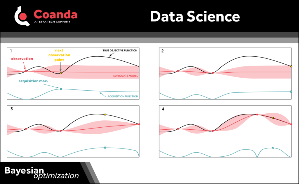
It uses a surrogate model for the objective function that also quantifies the uncertainty in that model (e.g., Gaussian process regression models are a common choice). Given observations (i.e., function evaluations), the surrogate model (posterior) is updated using Bayes rule. An “acquisition function” that is a function of the posterior is also defined; the acquisition function determines the next sample point from the parameter space. This process – updating the surrogate model and then evaluating the acquisition function to determine the next sample point at which to evaluate the objective function – is repeated until an optimum is reached.

The acquisition function is key to the method. The acquisition function uses all the past data/observations to pick the next “best” point in the parameter space at which to examine the objective function – the point it thinks is next best guess for where the optimum is. There are many different types of acquisition functions, some of these include
• picking the point that has the highest probability of improving the outcome,
• picking the point that has the highest expected improvement to the value of the outcome,
• sampling from the posterior distribution and picking the global maximum point from the sampled distribution.

You may have noted that, to optimize the objective function, Bayesian optimization now needs to optimize the acquisition function at each step. The key detail here is that the acquisition function, with the surrogate model, is a much simpler function that is very fast to evaluate and optimize. You could think of it as turning one expensive/hard optimization problem into many cheap/simple optimization problems.
For the right class of problems, Bayesian optimization can be a powerful method; it basically answers the question “how can we best use the info we already have to pick the next point we should examine”.