CFD Simulation of Inline Mixers
Posted on August 29, 2023 Computational Fluid Dynamics Mixing

This post was originally published in three parts which have been combined below.
Part 1
The in-line mixing of different streams is often a critical process for many industries such as chemical, pharmaceutical, and oil and gas. The primary goal is to achieve optimal mixing performance with a minimal pressure drop across the mixing device. Static mixers are commonly used in many applications due to their easy installation and low operating cost. However, selecting the best mixer for a given application can be challenging. The choice of mixer depends on factors such as flow rates, the properties of the fluids being mixed (i.e. the rheology of mixing streams), and available pressure drop. Two of the most widely used mixers are Kenics and Komax mixers, both of which are known for their ability to provide high mixing efficiency.
The Kenics KM mixer is composed of a series of alternating right- and left-hand helical elements that are mounted inside a pipe. These elements create mixing by increasing contact area and generating turning and shearing forces as the fluid streams flow through the mixer. On the other hand, the Komax mixer typically consists of a series of flat or helical vanes, stacked in series, which generates turbulence and creates a complex flow path for fluid mixing. In general, Kenics mixers experience a higher pressure drop compared to Komax mixers, due to the helical elements that create increased turbulence and shear forces.
In the next post, we will compare the performance of these mixers in the turbulent flow regime using a CFD simulation.
Part 2
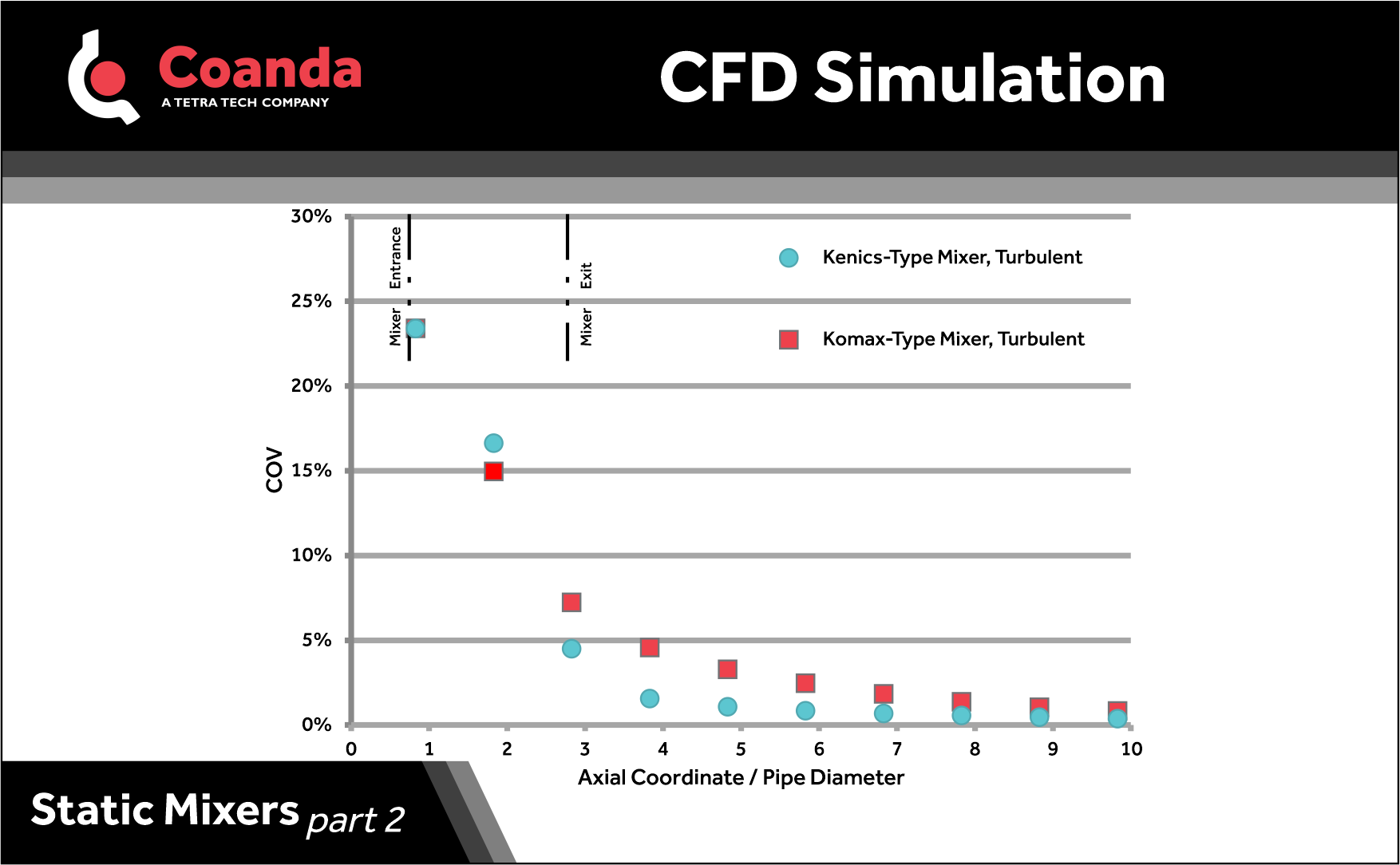
In the previous post, we discussed the general concept of in-line mixing and described two widely used mixers. The graph and figures presented below illustrate a performance comparison between Kenics- and Komax-type mixers for mixing Newtonian fluids in the turbulent flow regime. The scenario involves the injection of a liquid additive through a T-junction, which is intended to blend with a flow in the pipeline and the results are from a CFD simulation.
The coefficient of variation (COV), which represents the ratio of the standard deviation to the mean value of a variable, is commonly utilized to quantify the degree of non-uniformity within a distribution. In the top figure, a comparison is made between the COV values for the mass fraction distribution on cross sections downstream of the mixers. The pipe Reynolds number is 105, and for the assumed properties of liquids, the investigated Kenics- and Komax-type mixers show comparable performance. However, the Kenics-type mixer achieves a desired level of uniformity in a slightly shorter distance downstream of the mixer, although at the expense of a higher pressure drop. The pressure drop values are 1200 Pa for the Kenics, and 550 Pa for the Komax.
In the next post, we will compare the performance of these mixers in the laminar flow regime. A case study will illustrate the factors to consider when selecting the optimal mixer for a specific application.
Part 3
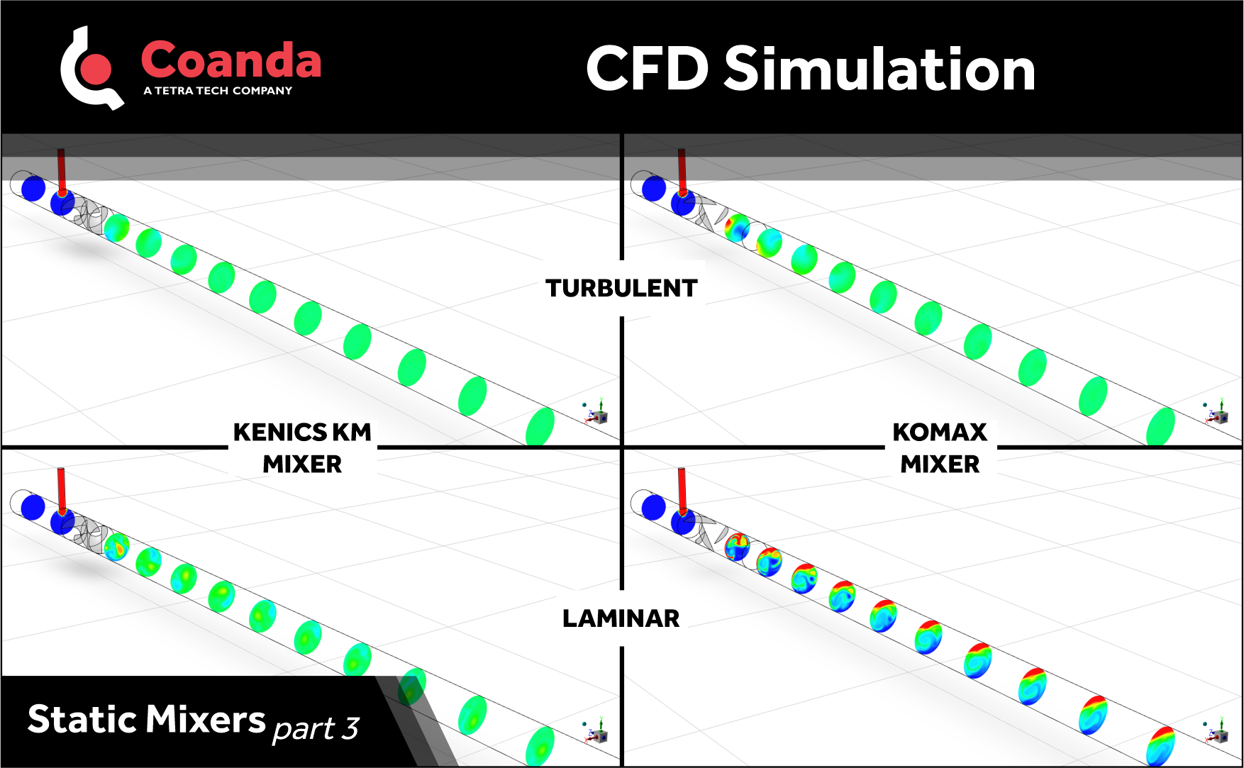
In our previous post, we explored a case study involving the mixing of Newtonian fluids and compared the performance of Kenics- and Komax-type mixers in turbulent flow using computational fluid dynamics (CFD). Now, we present a performance comparison between the two mixers in the laminar flow regime and include the results from the turbulent flow case for ease of comparison.
Considering a laminar flow condition with a pipe Reynolds number of 103, in which higher viscosity fluids are being mixed, the Kenics-type mixer demonstrates good mixing performance, with the COV values slightly higher than those obtained from the turbulence flow case. On the other hand, the Komax-type mixer is not able to achieve an acceptable mixing performance, as indicated by the COV values plateauing at a value of 15%. Similar to the turbulent flow scenario, the flow across the Kenics-type mixer experiences a higher pressure drop, ∆p Kenics = 1500 Pa, compared to the Komax-type mixer, ∆p Komax = 500 Pa. In this instance, the increased energy expenditure is indeed necessary to achieve the desired mixing performance.
The figures present the contours of additive mass fraction on different cross sections, with the colourbar clipped at 20% for clarity in the illustrations. It is evident that mixing is not satisfactory for the Komax-mixer in the laminar flow regime, even though both of them performed well in turbulent flow.
CFD simulations provide a reliable approach for comparing the performance of different mixers under various conditions, which helps with the selection of the optimal mixer for specific process conditions.