

X-Ray Systems & Analysis at Coanda
Coanda carries out a lot of physical modelling using carefully designed apparatus to test, validate, de-risk, or otherwise “figure out” some aspect of our clients’ processes. Usually, we can measure what we need with standard instrumentation, sometimes we build custom instrumentation, and sometimes we use x-ray systems.
X-ray has the advantage of being able to see into and visualize apparatus or processes that are opaque, cloudy, inaccessible, too fast, or (sometimes) transparent but with a density change – with the additional advantage that x-rays don’t bend (refract) like visible light when travelling through curved or angled surfaces. You can also work out density profiles and watch material degradation or settling on apparatus during operation without taking it apart for sampling.
Below we describe some of the x-ray systems we’ve accumulated over the years. They’ve all been integrated into various “live” apparatus or experiments as part of research programs and operate in purpose-built enclosures or bunkers (to eliminate unnecessary radiation doses to our operators). We also offer x-ray imaging and analysis of client samples or apparatus on a fee-for-service basis. We are not industrial radiographers – in the sense that we can’t certify a weld or casting – but if you’re a researcher who’d rather have the raw data than a certificate anyway please reach out or read on to see if we might be able to help (please also note that we do not x-ray people or animals).
Medical Source
For general-purpose x-ray visualisation we have a medical source that’s been modified to meet industrial safety standards. Our Poskom PXP-40HF has an energy range from 40 to 100 kVp and exposure range from 0.4 to 20 mAs. It’s good for visualising “people sized” objects. It can be used with any of our 14” x 17” flat panel detectors, which have a resolution of 160 to 270 microns, or our dental detector which has a ~26×35 mm size and 20 micron resolution.
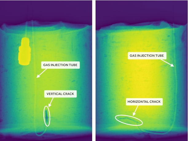 |
Figure 1 – Pneumatic-driven crack formation in a settled clay slurry, as imaged by Coanda’s Poskom PXP-40HF. In these false-colour images yellow/bright colours indicate a higher area density (of course, all x-ray images are false-colour images). Air was pumped into a thin tube (can be seen entering from the top and taped to the bottom of the bucket) until the backpressure dropped, indicating clay failure. Then we imaged the bucket from multiple angles to visualise the resulting cracks. Since the slurry is opaque, we would not have been able to see the structure of the failure and resulting pocket without x-ray. In this case the clay cracked and formed two narrow pockets at approximately right-angles to each other.
Pulsed Source
For things that happen fast, we’ve got a Golden XR200 pulsed x-ray source. This technology was actually developed as a lightweight and robust alternative to traditional high-voltage generation for light industrial and security use; as a byproduct the x-rays come out in 50 ns pulses. It operates at a fixed voltage of 150 kVp, there is no exposure adjustment (other than doing multiple pulses), and the exposure field is not quite as uniform as our other sources, but it can take crisp images of high-speed processes. We’ve used it to visualize mixed-phase nozzle sprays and fluidized beds as well as look at things like waves, free surface heights, slugging, and wall film thicknesses in multi-phase pipe flow. It can be integrated with any of our large panel detectors (see medical source info above), but not our dental detector.

Figure 2 – Gas bubbles breaking the surface in a column of fluidized sand, as imaged by Coanda’s XR-200. The fast x-ray allows visualisation of the structure of the fast-moving bubbles in an opaque medium. We’ve also used this setup to investigate and validate how various insertion probes affect the fluidized flow in their vicinity (fitting for this purpose visible near image bottom as a dense hexagon).
High-Power Fan-Beam Industrial Source
When accuracy matters, or for dense objects/apparatus, we’ve got a COMET MXR-320-HP/11-FB. It’s a high-power fan-beam industrial source paired with a line detector mounted on automated traverses. The source can do up to 320 kVp energy and 5.6 mA current at 100% duty cycle. The detector is 30 cm wide, oriented horizontally, with 100 micron resolution and the traverses have the repeatability to match. We have ~37 cm of vertical travel and almost 2m of horizontal travel on the traverses. A typical scan time with this system is a few minutes, but for dense/thick materials (we’ve done up to 4” of steel) we can do a scan over several hours. For lightweight materials/apparatus we can produce x-ray “videos” with a framerate as fast as 1 Hz.
It’s worth discussing how a traversing fan beam with line detector system works, and what the advantages are. In typical use we orient the source and detector directly across from each other inside the bunker; the detector is sensitive over a narrow horizontal strip, and the source emits a narrow “fan” of x-rays illuminating just the detector active area. The source and detector then traverse together vertically to form an image (see Figure 3). This has several advantages over taking the image “all at once” using a flat panel and cone-beam source.
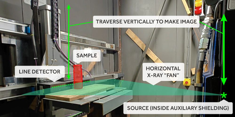 Figure 3 – Annotated photo of Coanda’s traversing fan beam system
Fan-Beam Advantage: Secondary Scattering
Radiography forms an image when some fraction of the x-rays gets absorbed by the object. The more material, the more absorption, so you can work out the area density from the reduction in x-rays detected. However, many x-rays are not simply “absorbed” by the object being imaged – some scatter. Many of those scatter generally forwards, but some scatter and re-scatter at other angles too. With a panel detector these scattered x-rays are also detected (although they can be reduced somewhat by grids of heavy material that try to restrict the entry angles to the detector). These “extra” counts interfere with an accurate calculation of the density of the object under study. For thick, high-density, objects they might even drown out the desired signal entirely. See Figure 4.
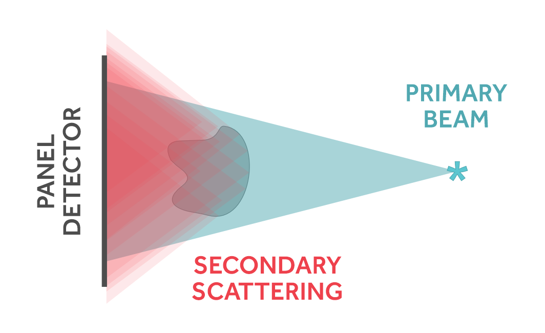
Figure 4 – Conceptual sketch illustrating secondary scattering being detected with a flat panel detector. Most of the forward-scattering is detected.
With a fan-beam system you can apply heavy collimation to both the source and the detector. The source only emits the x-rays that are being “used” by the row of pixels you are currently exposing, and the detector is only sensitive to x-rays coming in from that specific direction. “Extra” counts from secondary scattering are almost completely eliminated. This allows an accurate calculation of the area density of the object. It also allows for extremely long exposures in situations with low count rates where secondary scattering around the bunker would otherwise drown out the signal. See Figure 5.
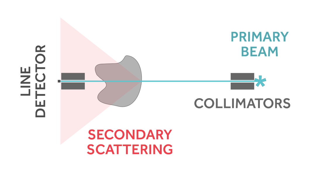
Figure 5 – Conceptual sketch illustrating secondary scattering being eliminated by a traversing fan beam system with collimation. In this sketch we’re looking at the system “edge on” so the line detector appears as a point, and the fan of x-rays appears as a line. Almost none of the secondary scattering is captured by the detector.
Fan-Beam Advantage: Geometry
With 2D panel x-rays (and regular photos) there are geometric effects because each pixel represents a different angle. For example, if you take a picture of a jar, looking “straight across” at the middle you’ll actually be looking down on the bottom from above and up at the top from below. So, the base and the lid look like ovals. This doesn’t seem unusual, because it’s how we’re used to looking that the world, but it means that information from different elevations is superimposed on top each other (see Figure 6). But if you want to calculate density as a function of elevation you can do a much better job if each row of pixels represents a unique elevation. With a traversing fan beam that’s exactly what you get since it’s always measuring straight across, moving the source and detector together (see Figure 7).
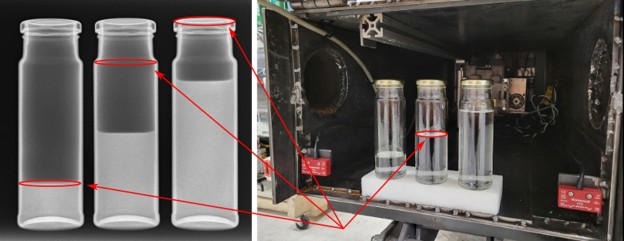
Figure 6 – X-ray and regular images of 3 jars of water, taken in Coanda’s high speed pipeflow x-ray enclosure. Due to the angles horizontal parts of the jars that aren’t directly in-line with the camera (or x-ray source/detector) appear as ovals in the images.
Fan Beam Advantage: Example on tailings jars
As an example highlighting these two advantages let’s go over the process of measuring the density profile of some geotechnical samples after they were spun in one of Coanda’s geotechnical centrifuges. Looking at the x-ray image, Figure 7, we can see that with the traversing system the lids and bases of the jars are now completely flat – each row of pixels holds information from only a single elevation.
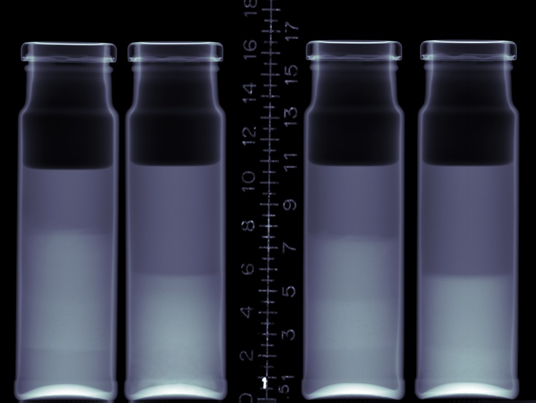
Figure 7 – X-ray image of centrifuge sample jars taken with Coanda’s traversing fan beam system. Each row of the image represents a single elevation, easily seen by comparing the lids to Figure 6.
Due to manufacturing tolerances, the wall thickness on the jars is not very uniform. You don’t see it by eye, but it will make a big enough difference in the absorption that we’ll notice it when calculating the density. We do some image analysis to pick out the edges of the glass walls in the image; this lets us calculate the wall thickness and inner diameter as a function of height. In Figure 8 we show some diagnostic plots from the process showing the edges and dimensions as found. We then take a second x-ray with the jars rotated 90 degrees; we can use the wall thickness and ID from one to calculate the material density from the other, the results for jar A are shown in Figure 9.
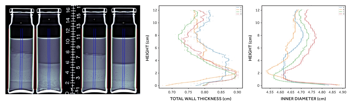
Figure 8 – Left edge boosted version of Figure 7, with thin red lines showing the external edges of the jar, green lines showing the internal edges, and blue lines showing the strip down the middle used to calculate the density. With edge-boosting (more on that later) the different layers in each sample are more clearly visible. Centre and right show the wall thickness and internal diameter as a function of height as used to calculate the material density from the absorption.
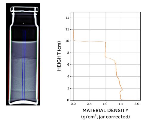
Figure 9 – Material Density as a function of height for jar A from Figure 7/Figure 8, as calculated from x-ray absorption assuming uniformity across the inside of the jar. (Note that the height scale in this figure sets zero as the bottom of the inside of the jar; the x-ray ruler in the x-ray images is placed with zero at the bottom of the outside of the jars). Now we see the density profile associated with the layers. You can see the release water (at the top, density 1 g/cm3) as well as the fact that the density profile is not what you might naively expect – some material near the bottom of the jar settled more quickly, but ultimately consolidated to a slightly lower density than the material that settled on top. This is something you’d only be able to see by either radiography or a time-consuming dissection of the sample.
Why Area Density?
Maybe the most frequently asked question I get from people looking carefully at x-ray images is “Why is your axis/colour-scale in area density? Shouldn’t it just be density?”. Even though I think people intuitively know it’s area density (or something like it) it’s easy to think it might be density at first glance, especially if density is what you really wanted to know in the first place.
By means of example, let’s take two loonies and x-ray them so that they are slightly overlapping. The coins have the same density, but the overlapped region should absorb more x-rays because there’s twice as much material in the way. The absorption depends not just on the density, but also the thickness of material. Density times thickness will give you an area density.
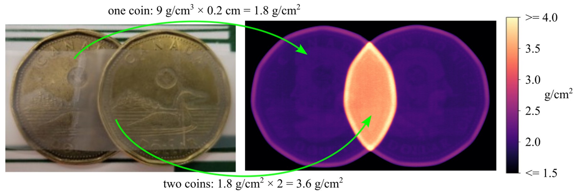
Figure 10 – Two loonies, shown as both regular and x-ray images. The overlapping part of the coins absorbs more x-rays and shows up as having double the area density in a calibrated x-ray image since it’s twice as thick.
Of course, what we really measure is x-ray absorption… but if you have calibrated your source and detector (and we generally take a calibration image along with every x-ray we take) you can work out the area density, assuming that the x-ray cross section is the same for your calibration plates as the atoms in your sample. For “normal stuff” (the first couple rows in the periodic table) this works well enough, but higher-atomic-number materials do absorb substantially more x-rays per unit mass than lighter elements, especially at lower x-ray energies. This is why lead makes such good shielding – not only is it dense, but it also absorbs way more per unit mass. You can look up the absorption for any element, compound, or mixture as a function of energy in tables using NIST’s excellent XCOM web tool.
Squeezing Out Detail With Edge Boosting
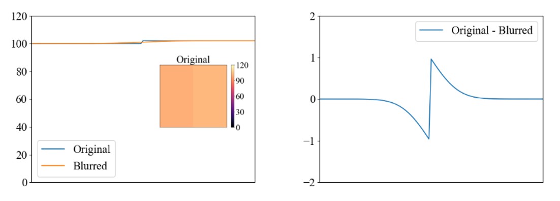
If we look at the coin image above, with colours based on area density, you can just barely make out the design on the coin. The information is there, but the changes in thickness are tiny compared to the thickness of the coin so it all shows up as almost the same colour. If we want to see this detail we can play some tricks to help it stand out. Most often we would do an edge-boost (Figure 11). Essentially by subtracting a blurred version of the image from the image you end up with an “edges only” image: uniform regions go to zero and edges end up as little wiggles. Then you can add that “edges only” image back onto the original to get the overall value of smooth regions in the same ballpark as the original. You can play with the size of the blur and the relative magnitude of the “edges only” image until you see the detail you’re looking for. A series of plots illustrating the steps in 1D is shown in Figure 12.
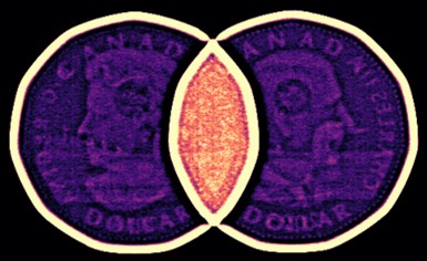
Figure 11 – An edge-boosted version of the coin x-ray image from Figure 10. The colour-scale no longer directly shows the area density (the edges of the coin are off-scale now, for example), but the small details in the coins’ design are more clearly visible. Of course, with an x-ray, you see both sides of the coin!
 |
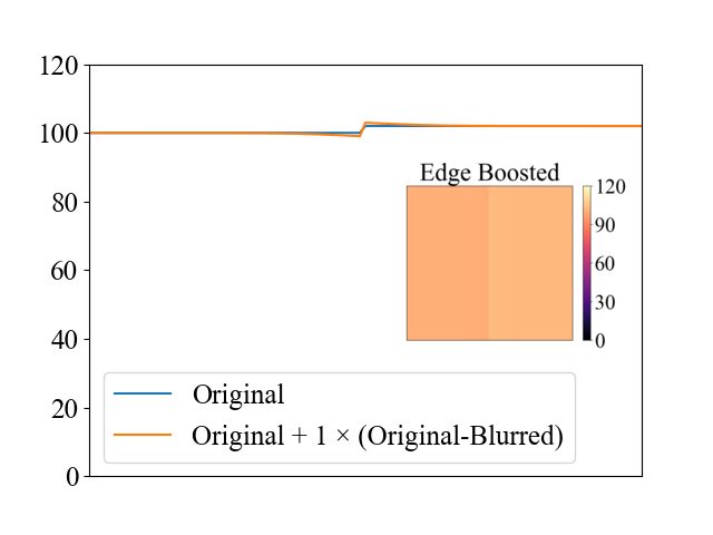   |
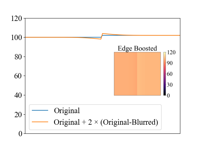
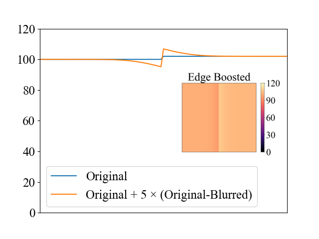
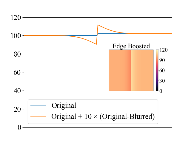
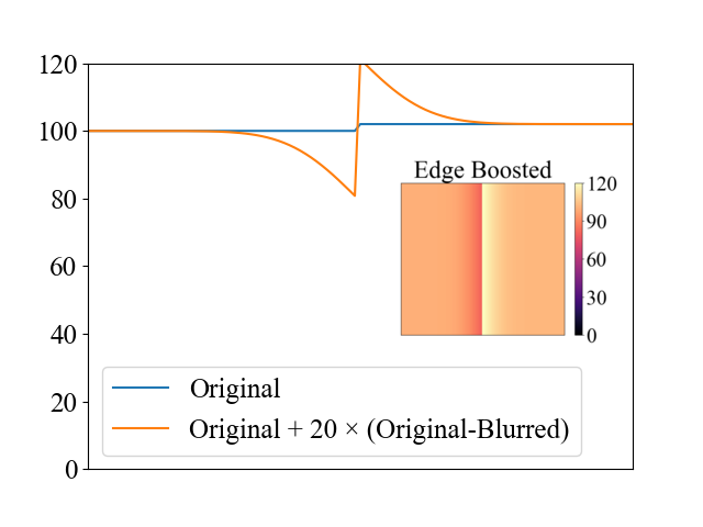
Figure 12 – A 1D example showing the steps of the edge-boosting method. A small edge in the middle is scarcely visible as it’s small compared to the overall value of y=100, but mixing the original function with an “edges-only” (original-blurred) turns the small step into a large easy-to-see feature.
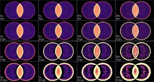
Figure 13 – Edge boosted versions of the coins image, for different magnitudes and kernel diameters. In this example the kernel used for the blur is a symmetric gaussian, but it could be any shape.
Another Analysis Trick: Difference Images
Often, we’re more interested in small changes against a large background – maybe you have a catalyst deposited onto the inside of an assembly and you’re worried about degradation, or maybe you have small channels carrying fluids and are worried about bubbles. In this case we can set up the experiment inside the bunker, x-ray it in the reference condition, and then again during the experiments. Looking at the difference images the apparatus itself “disappears”, leaving only the changes. Some examples are shown in Figure 14 and Figure 15.
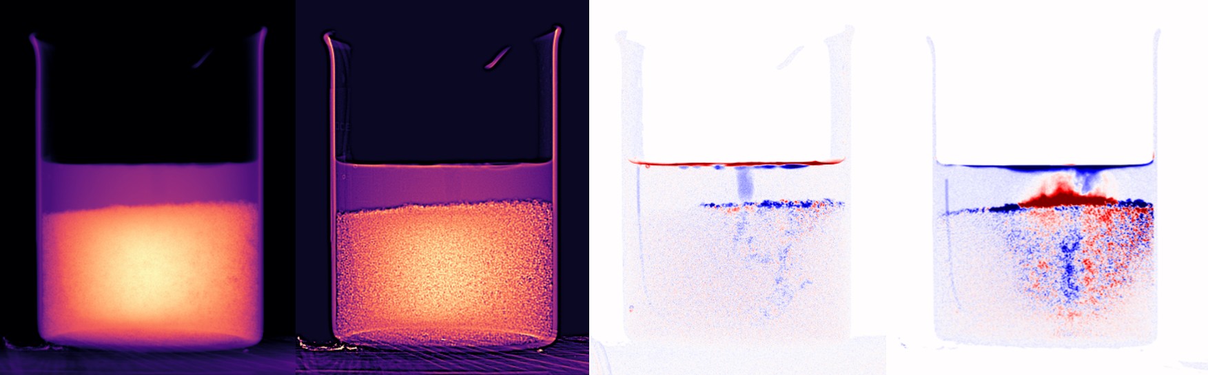
Figure 14 – Bubbles rising through a bed of glass beads in a beaker of water. In the density image (left) it is difficult to make out the beads or the bubbles. Edge-boosting (centre left) helps show individual beads (as well as grains in the wooden table), and the bubble rising through the water is more visible. In the difference image (centre right) blue represents a reduction in mass while red is a gain in mass compared to the bed with no bubbles. Now the wandering path the bubbles are taking through the bed can be seen. You can also see that the tiny tube delivering air was filled with water in the reference image, as it now appears as a light blue (mass loss) line down the left inside edge of the beaker. With a higher gas flow rate (right) the beads shift – the extent of this cone can be seen as the region with red and blue “noise”; slumping at the edges of the cone from the original height of the beads shows up as dark blue on the top, and a rise in the middle shows up as red.
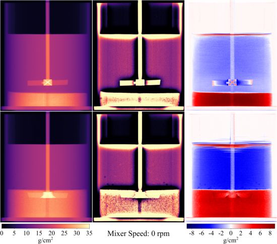
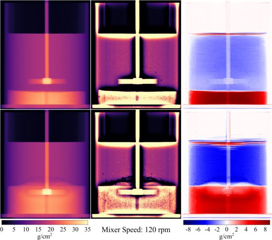
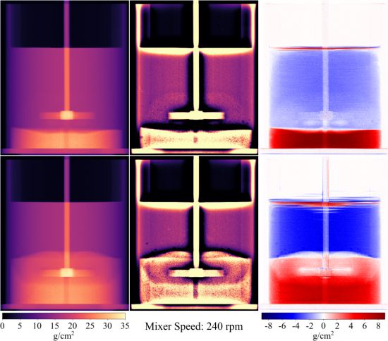

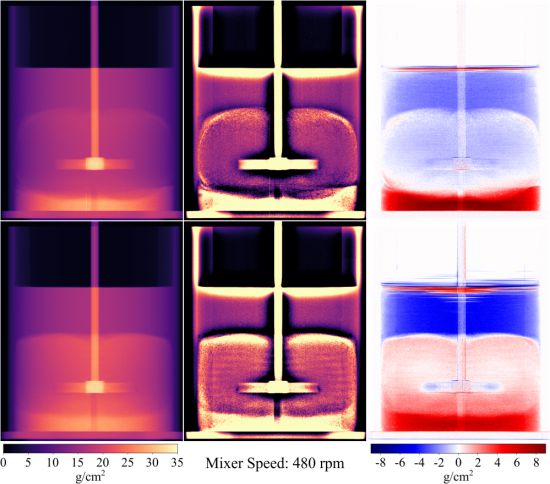
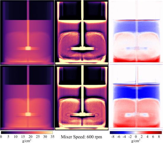
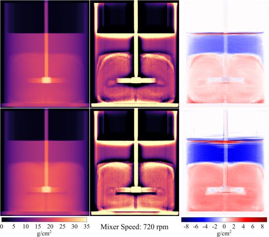
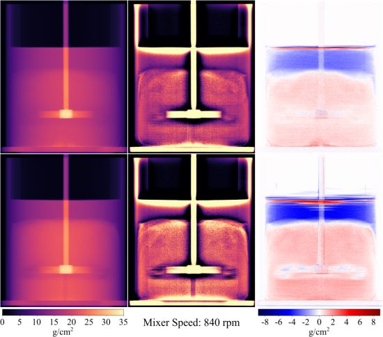
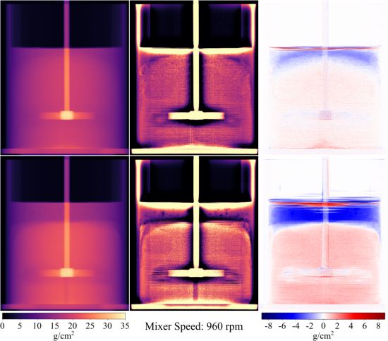
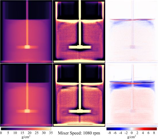
Figure 15 – Cavern mixing demo. Fine solids (10% by volume, top, and 20% by volume, bottom) are mixed into a Carbopol solution. Carbopol is a yield-stress fluid, a type of non-Newtonian fluid that will not flow until subjected to a minimum shear stress. This means that during mixing the fluid will divide itself into distinct regions: the “cavern” around the impeller, where mixing occurs, and a stationary region surrounding the cavern that does not mix (at least until the cavern expands to fill the container). Here we show area density (left) edge-boosted (center) and difference (right) x-ray images of the process of mixing solids into the Carbopol. The reference image for the differences is fully mixed. The horizontal lines near the top of the liquid (especially visible in the difference images) occur because the free surface is moving at a similar speed compared to the scan rate on the traversing fan beam system, so the free surface is in a different location for different rows of pixels. The impeller shaft and baffles appearing slightly “white” in the difference images is not an error – their mass is subtracted away and there’s less fluid to change density in those locations (because some of the volume is occupied by the mixer and baffles) so they appear lighter.