Magnetic Flow Meters explained
Posted on July 6, 2022 Instrumentation and Equipment Design

This post was originally published in four parts which have been combined below.
Part 1
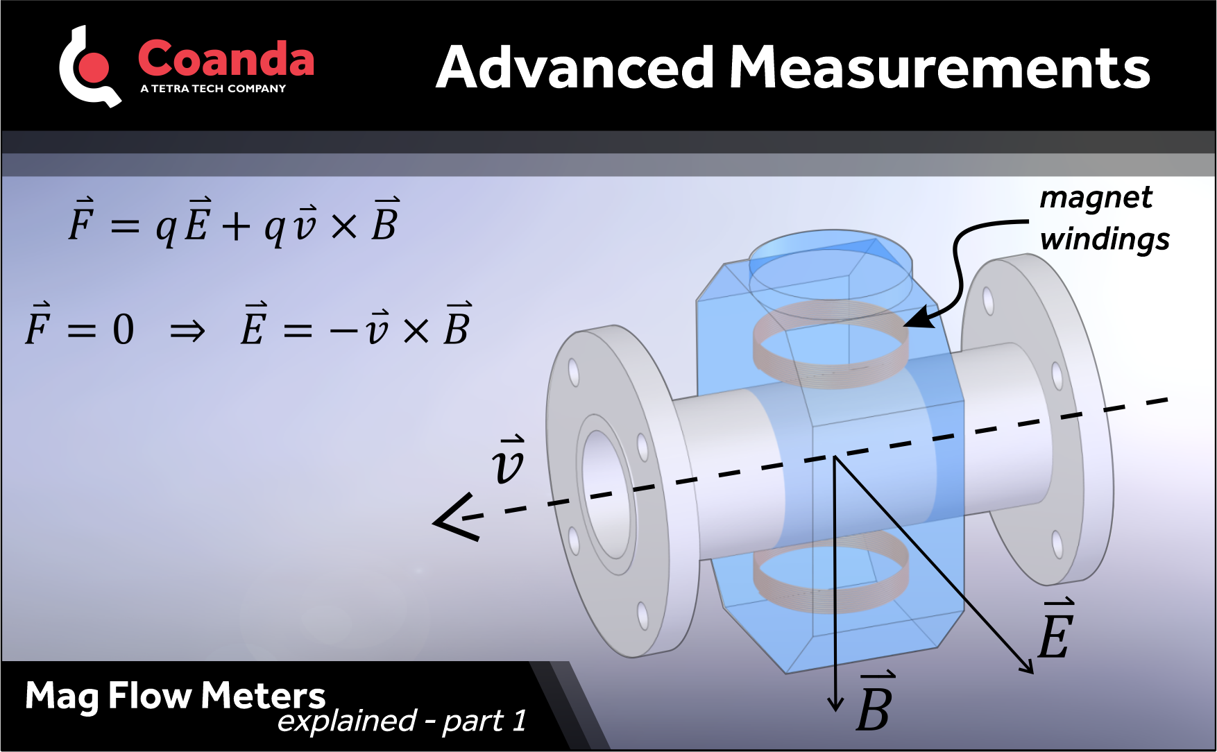
Electromagnetic flow meters, or mag meters, are the most robust and generally applicable flow meters for slurries. Still, they do not work in all scenarios and understanding the physics of the measurement is key for anticipating and avoiding errors and failures.
The mag meter creates a magnetic field across the pipe flow and measures the voltage perpendicular to both the pipe and the magnetic field. Every charge going through the pipe experiences the Lorentz force. Assuming flow is uniform, and charges can move in response to the force, i.e., the material is conductive, they will find equilibrium within microseconds. Equilibrium means no net force, so we get an electric field that is equal and opposite to the cross product of the flow velocity and the magnetic field. The cross product is perpendicular to its arguments; in-line with the voltage measurement.
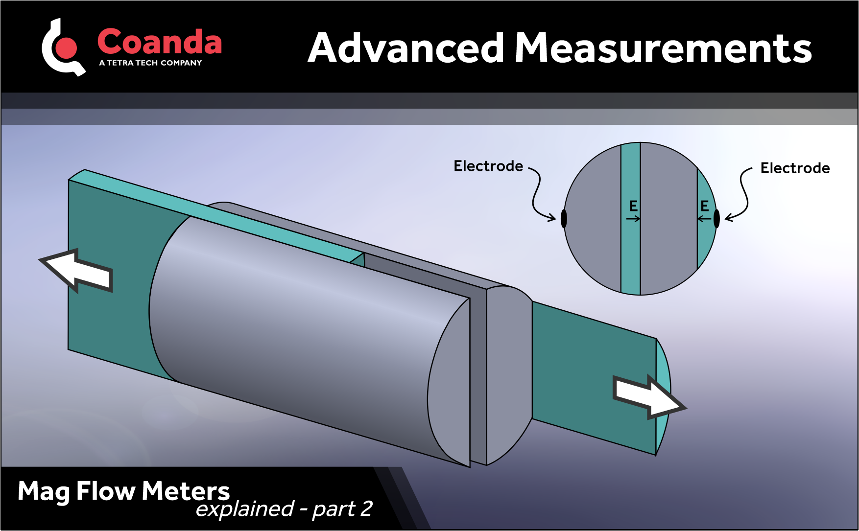
A path integral of the electric field between electrodes gives the voltage. With a known magnetic field and pipe diameter, the flow is found.
Note that the conductivity of the fluid does not appear in the equation. Conductivity only affects equilibration time, not the final voltage.
In the next post, we start to explore where problems might arise.
Part 2
Last time we looked at the measurement principle of mag meters, and here we’ll explore the effects of flow distribution.
The flow distribution illustrated below would be difficult-to-impossible to create in real life, but it provides a clear illustration of the meter’s sensitivity. In this hypothetical example, most of the liquid is stationary but there are two equally thick layers moving in equal and opposite directions (shaded). Since the voltage measured is a path integral, the contributions from each layer cancel out and the mag meter reads no flow. The layers shown have different cross-sections, so the actual net flow is distinctly non-zero.
Placing a mag meter too soon after an elbow or other piping change will cause less dramatic but still significant errors.
In a developed flow of a homogenous material, the velocity will depend only on radius. The distribution does change as a function of Reynolds number, but the overall effect is relatively minor. Meters are typically calibrated in the turbulent regime and are still within a couple of percent of reading in laminar flow.
Large errors can occur when there are multicomponent flows. Stay tuned.
Part 3

Last post, we looked at the effect of flow distribution on mag meter readings. This example shows that while the mag isn’t sensitive to conductivity of a uniform fluid, conductivity differences in inhomogeneous flows matter.
Maintenance staff are working to flush out a large horizontal pipe filled with brine with a density of 1050 kg/m3 using fresh water. The brine pipe has a mag meter on it. They turn on the water and see an initial surge of flow on the mag meter, but the mag meter’s display shows a steadily dropping flow. The staff watch, bewildered. What is happening?
When the water is first turned on, brine is displaced from the pipe at the rate that water is added, and the mag meter reads correctly. Since the pipe is large, the net velocity is too small for good mixing, resulting in a stratified flow, with near-stationary brine in the bottom half of the pipe, and buoyant, faster-flowing water on top. The magnetic field interacting with the brine produces a minimal electric field. The moving water would in principle create a voltage, but the brine is hundreds of times more conductive, shorting out the contribution from the fresh water.
The next and final post in this series touches on other challenges.
Part 4
Last time, we looked in detail at a scenario where a mag meter can underreport a flow by a huge factor. Here we’ll look at a few other common problems.
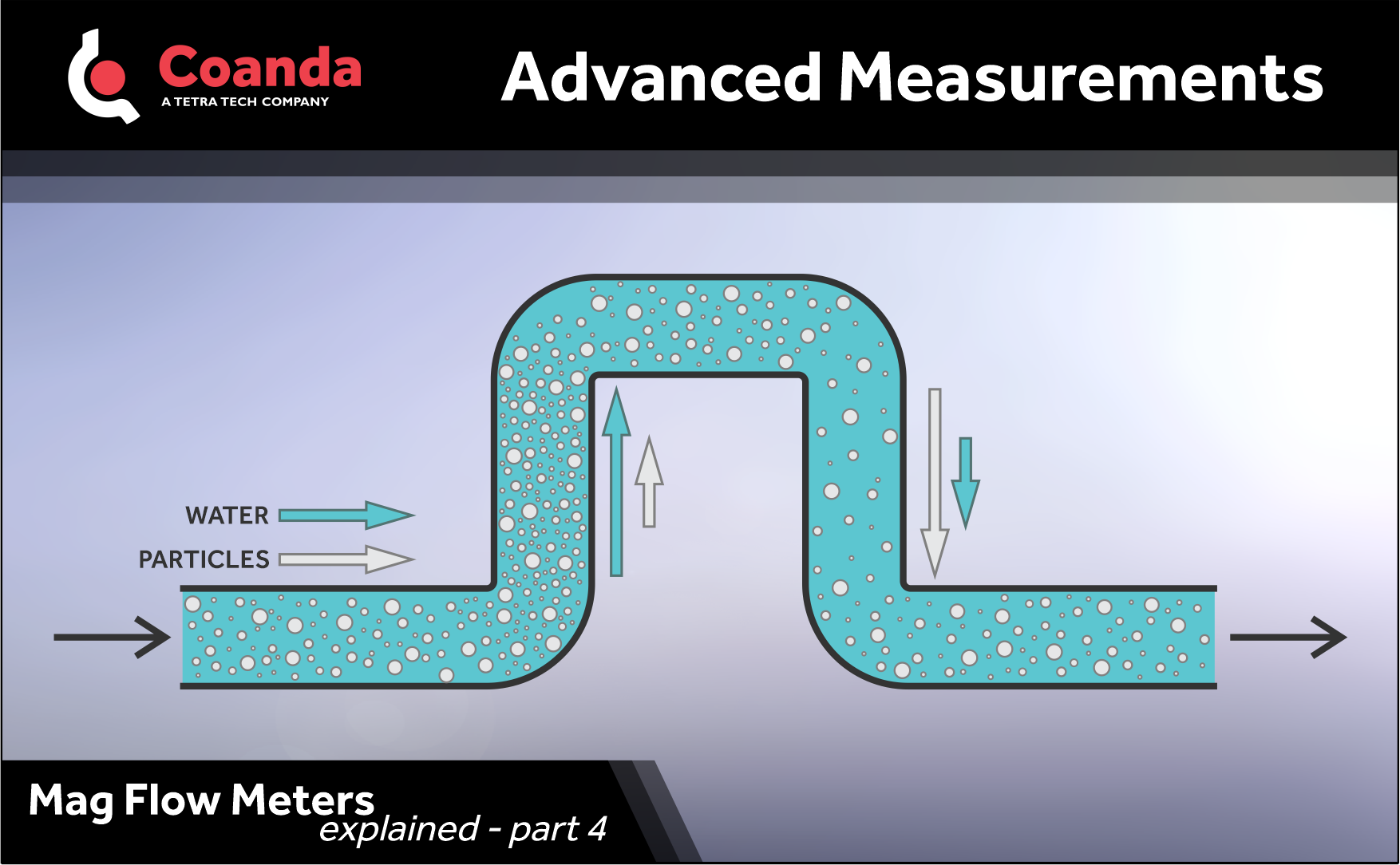
Vertical flow with conveyed solids: a slurry of non-conductive dense solids flows up through a vertical pipe. The solids settle relative to water, creating a velocity mismatch. Since the solids don’t conduct, the mag meter sees only the water and reports the wrong average flow.
Fouling conditions: The measurement electrodes become coated with an insulating foulant. The mag meter can no longer read a voltage and either reads no flow or throws an error, depending on the model.
Bubbles: A mag meter needs a full pipe to give an accurate volume flow rate. Air at the top of a horizontal pipe can be detected with an empty pipe detection electrode at the top if the mag meter is equipped. If the air is entrained, though, this isn’t detected, and the flow rate is over-reported.
There is no universal solution in slurry flow measurement. Mag meters are often the best option, but understanding their limitations is key to a successful implementation.