Data Science – Non-parametric Regression
Posted on March 17, 2022 Big Data Machine Learning & AI

This post was originally published in two parts which have been combined below.
Part 1
Gaussian Process Regression – Non-Parametric Regression
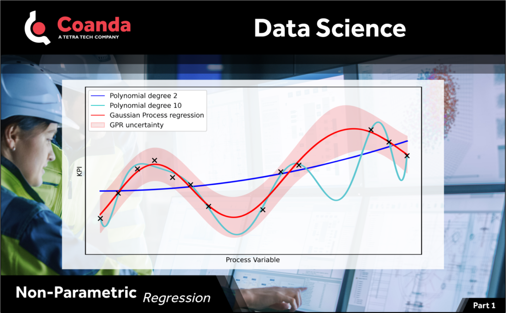
Often for data that is collected from industrial processes, the functional relationship describing the data is unknown. An example of this could be a key performance indicator (KPI) which is measured as a function of an adjustable process variable.
We may want to interpolate the measured data to predict the KPI at new process conditions or to perform some other type of analysis. One way would be to fit a polynomial to the data, but this approach suffers from the drawback that a high-order polynomial will go through most, if not all, the measured data points but will oscillate wildly in between data points. A low-order polynomial on the other hand may not fit the measured data well.
Often a better approach is to use a non-parametric regression method instead, such as splines or Gaussian Process Regression (GPR). GPR is particularly attractive as it allows us to fit a function of arbitrary complexity to the data, making use of any general knowledge that we have of the process, while also naturally accounting for any noise or uncertainty in the data. In the next post we’ll describe how GPR works.
Part 2
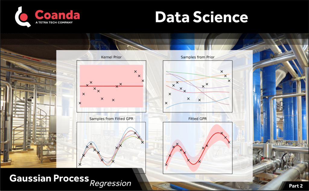
Gaussian Process Regression (GPR) allows us to fit a function of arbitrary complexity to data while making use of any general knowledge we have about the behavior. For example, even though we do not know the functional form, we may have some general knowledge about the data from the governing process, e.g., that it is smooth or includes a trend. As well, GPR provides a natural way to account for uncertainty in the data and fit. It achieves all this through the use of a kernel function which models the covariance (joint variability) between data values. The form of the kernel determines the general properties of the function such as smoothness or trends and different types of kernels can be combined to produce properties which are tailored to the problem at hand. The kernel is then fit or conditioned on the data to produce an infinite set of functions which have the general properties given by the selected kernel and pass through (or near) the measured data. From this infinite set of functions, we can determine a “mean function”, which is akin to the best fit curve, and estimate the uncertainty in the fit around this mean function.