News + Publications

The residence time distribution (RTD) of piece of fluid-handling equipment like a tank, pipe, or reactor describes how much time fluid spends inside. For example, in a batch mixer or ideal plug-flow reactor, all of the fluid spends the same amount of time in the vessel. If we plot a distribution of fraction of fluid vs. the amount of time spent in the vessel, we get a spike corresponding to the residence time, as shown below (left). On the other hand, for fluid flowing through an ideal continuous stirred tank reactor (CSTR), some of the fluid that enters the tank goes through immediately (because the tank is perfectly mixed), but some spends a longer time. This means there is a distribution of time spent in the reactor over all of the fluid elements passing through, also as shown below (middle).

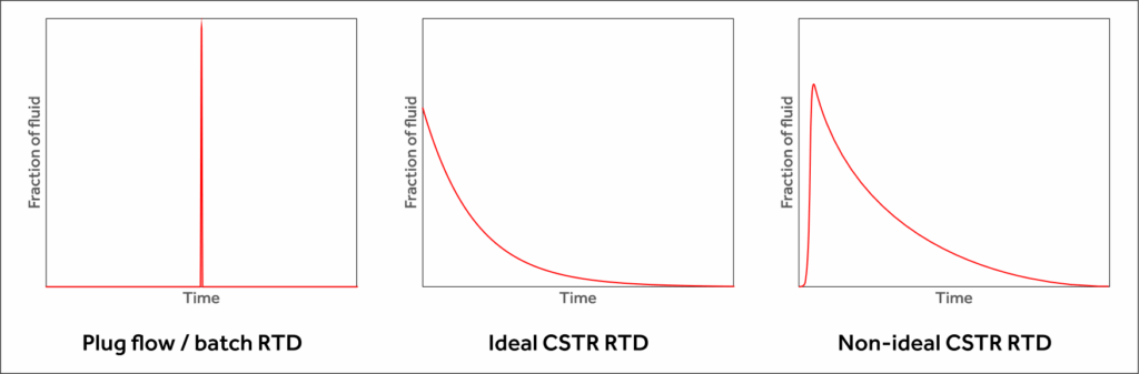
Real residence times are not ideal like the ones mentioned above – e.g. mixing is never perfect, so there is always some transport time between inlet and outlet. The effect of non-idealities like this can be seen in the non-ideal CSTR RTD shown above (right). An advantage at looking at fluid behavior in a process in terms of RTDs is that real residence time distributions can be measured using various tracer methods, or sometimes by looking at the response of a process unit to changes in conditions during operation. This post from a while ago describes how that is done: Residence Time Distribution Measurements

Another advantage of describing processes in terms of residence time is that both measured and ideal RTDs can be conveniently described mathematically. This lets you do things like combine RTDs for individual process units to model a larger system, or build up a complicated RTD from simpler ones. This is done through a mathematical operation called convolution. While we won’t go into the details here, this operation ends up being numerically convenient for implementing these calculations, as it can be done using Fourier transforms, which are ubiquitous and well-supported in many programming languages.

An example of the kind of behavior that can be modeled using RTDs is the ‘ringing’ observed in the concentration profiles within a recirculation loop. This sort of ringing can occur when a plug flow, or process unit with a plug flow component in its RTD, is part of a loop, as in the schematic below. This could be, for example, a stirred tank in a loop with a plug flow reactor. If a tracer chemical is injected into the loop for 5 seconds, its concentration at various points shows an oscillatory behavior due to the lag in the system. This can be captured in an RTD model as shown below. Concentration units are arbitrary for this example, and it is assumed that the amount of tracer is small compared to the amount of fluid in the system.

The blue line in the plot above is the concentration of the tracer at point A. Due to the tracer injection, it jumps up immediately as the tracer injection starts. At the 5-s mark, the tracer injection stops, and there is no longer any difference between the concentrations at points A and C, so the blue line follows the green line in the plot exactly.

There is initially no change at point B because of the lag in vessel E1. Once the tracer breaks through E1, the concentration into and out of vessel E2 (B and C, respectively) start to increase. The concentration at A also starts to increase after breakthrough, because tracer is now being added to the fluid containing recirculated tracer. The oscillations occur as the fluid passes through the lag in E1. The final steady concentration is lower than the peak value observed, reflecting the dilution of the tracer once it is evenly distributed in the system.

Modeling this sort of behavior could be complicated using a first-principles approach, more so if non-ideal aspects of the system had to be considered to capture real behavior. Using RTDs simplifies the description of the system and would allow for measured data to be incorporated or approximated using combinations of RTDs.