High Speed Multi-Channel Conductivity Meter
Posted on May 2, 2023 Instrumentation and Equipment Design

This post was originally published in two parts which have been combined below.
Part 1
For many of the experiments Coanda performs concentration can be associated with a key performance indicator – for example uniformity in mixing or the breakthrough and residence times. Injecting a tracer and monitoring its concentration is an ideal way to study such systems. Salty water is cheap and non-hazardous and conductivity meters are readily available – making it an excellent tracer in water-based experiments.
So why is this post titled “custom instrumentation”? Well, most readily available conductivity meters are designed to measure salinity quite precisely for environmental monitoring and suffer from several downsides when used for our industrial process modelling experiments: they are typically quite slow, the probe element may be expensive and large enough to interfere with flow, they may interfere with each other if used in close proximity, and many don’t deal gracefully with a metallic pump in the system running off a variable-frequency drive. They also usually have features that aren’t necessary, such as correcting for temperature, converting to total dissolved solids (assuming a particular salt distribution), or being designed for handheld field use.
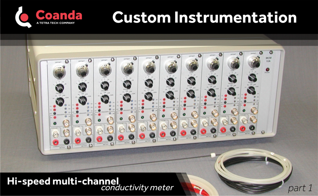
For these reasons one of Coanda’s earliest custom instruments was a fast response multi-channel conductivity meter, as seen in this photo pulled from the Coanda archives. It was originally developed by Coanda’s founder, Darwin Kiel, in collaboration with David Wilson at the University of Alberta, and further refined with Rex Britter and John Mumford at the University of Cambridge. These devices have provided valuable data related to scalar mixing and dispersion in many experimental studies over three decades at Coanda and elsewhere.
In our next post we’ll go over the more recent redesign by Coanda’s Instrumentation Department, highlight the performance achieved and how it was done.
Part 2
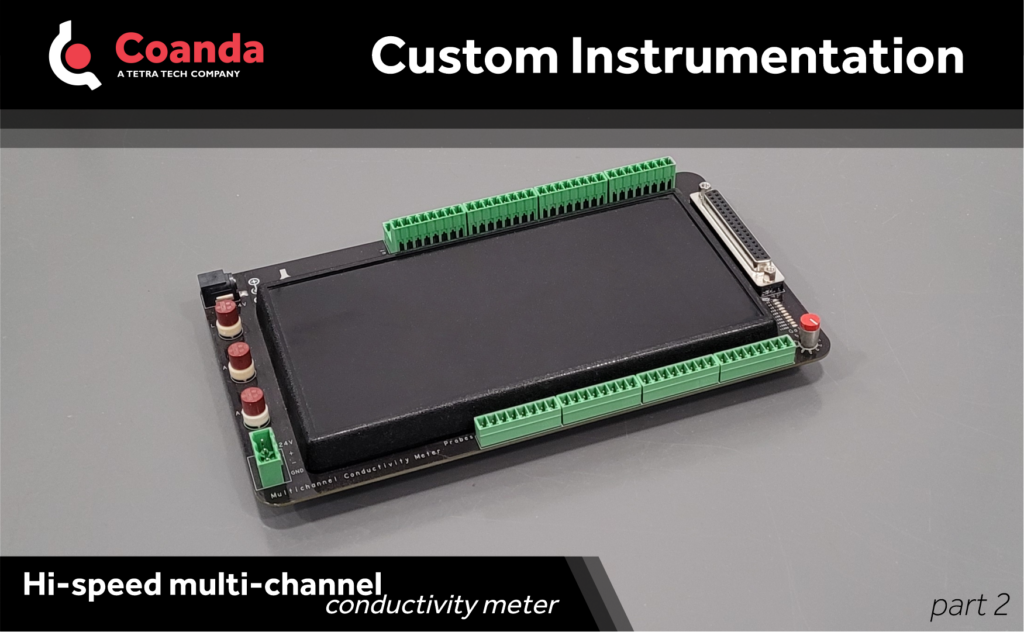
In the last post we motivated why Coanda would bother to develop an in-house conductivity meter: developing instrumentation is fun, but if a suitable instrument is commercially available, we’d prefer to just buy it. Here we discuss the Coanda Instrumentation Department’s redesign, highlight the performance achieved and how it was done. Aside from being physically smaller it has a number of advantages compared to both traditional systems and the original design; it’s been in service for about 5 years.
A key conceptual carryover from the original design was to use ordinary solid-core wire for each “probe”. If you do the math you’ll discover that, with a large ground plate for the return, only the conductivity within a few tip diameters really matters. The ground plate (or simply a metallic vessel) can be shared between all probes. This brings the cost of outfitting a rig with probes essentially down to the labour required to install them; it’s also easy to get a wire into tight places without interrupting the flow. Not only that, but aspects of the measurement can be customised with different diameter wires – larger wires increase signal in low-conductivity solutions and average out over a larger volume, which might be desired if there are non-conductive particles in the water. If a large ground plate is not possible one can also use concentric needle electrodes (as sold for medical purposes).
Over to the redesigned electronics driving it: The 5 kHz drive frequency is slow enough to measure DC conductivity, but prevents plating and is fast enough that the channels can be multiplexed: each probe is driven sequentially for just long enough for the measurement to settle. This eliminates crosstalk between probes and is still fast enough to measure all 32 channels in about 50ms. A phase-lock multiplier drastically reduces noise pickup as well as capacitive coupling to ground, while dummy channels on the opposite side of the PCB mitigates the effect of thermal gradients. This, along with a few other details and modern components, allows a useful range from 10 nS to 1.5 mS.